Camera¶

class pyvsim.Toolbox.Camera[source]¶

This class represents a camera composed of a body (used only for display), a sensor and a lens, therefore it is an assembly.

The main functions of this class are driving the sensor and the lens together, so that the user can call more logical functions (such as initialize) instead of using a complicated series of internal functions.

The camera creates a mapping of world coordinates into sensor coordinates by using direct linear transformations (a pinhole model). Lens imperfections and ambient influence can be modeled by using several DLTs (which is controlled by the parameter mappingResolution).

The reference points and origin of used in the development of this class are shown in the figure below:

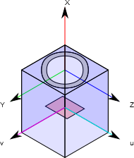
The following points are noteworthy:

• The camera points at the \(x\) direction. \(y\) is pointing up and

  \(z\) points to the right.

• The origin of the camera is the center of its flange (the connection with its lens)

• The sensor is positioned at a negative \(x\) position

Methods

bounds[source]¶

This signals the ray tracing implementation that no attempt should be made to intersect rays with the camera

circleOfConfusionDiameter = None¶

Allowable circle of confusion diameter used for depth of field calculation, standard value - \(29 \cdot 10^{-6}m\)

color = None¶

Camera body color (for plotting only)

detmapping = None¶

Determinant of the mapping matrices (used to verify if the \((x,y,z)-(u,v)\) mapping mapping goes from a right handed coordinate system to another right handed, or there is a flip

dimension = None¶

Camera body dimensions (for plotting only)

dmapping = None¶

Derivative of the \((x,y,z)-(u,v)\) mapping

initialize()[source]¶

This function calculates the camera field of view and its mapping functions to relate world coordinates to sensor coordinates. This should be called whenever the ambient is set up, so the camera can be used for synthetic image generation and displaying.

The procedure is capable of estimating the focusing region by using a hybrid ray tracing procedure. This is needed because the conjugation equation ( \(f^{-1} = p^{-1} + {p^{\prime}}^{-1}\) ) is not capable of representing the cases where there is a refraction between the measurement area and the camera.

The approach consists then on taking the theoretical focusing points (as calulated by the conjugation equation) and using them to calculate initial vectors (departing from the exit pupil) for a ray tracing. The focusing point is then the intersection between the rays. The procedure is shown in the figure below:

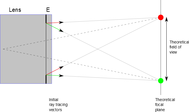
The program implements 4 rays per point (departing from directions \(y,z,-y,-z\) in the camera reference). This is sufficient for most cases, and is just an approximation in the case the refracting surface is not perpendicular to the camera axis (except the case when it’s inclined in the cameras \(y\) or \(z\) axes only), because in this case astigmatism is present.

The line intersection is performed between the rays starting from \(y,-y\) and \(z,-z\) separately, which generate the points denominated VV anh VH. When these points do not coincide, the system is astigmatic.

This approach is in fact adapted to consider the depth of field. The extension is natural and involves calculating the theoretical forward and aft tolerances for focusing (this is a funcion of the parameter circleOfConfusionDiameter). The procedure is shown in the figure below:

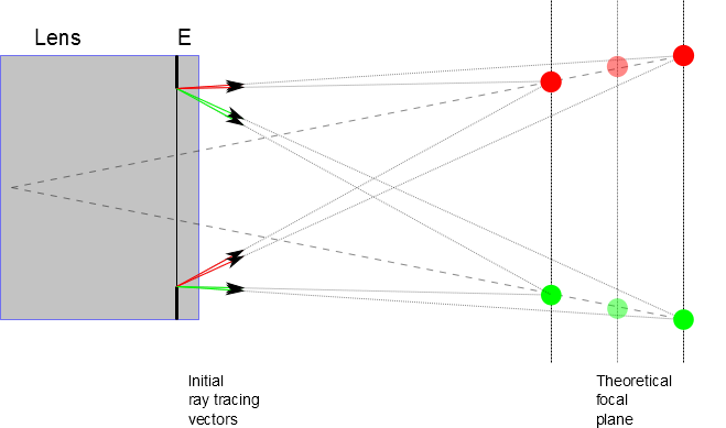
For each subfield (which number is defined by the mappingResolution property) 8 points are calculated. These points are then used to derive a direct linear transformation (DLT) matrix relating the world coodinates to the sensor coordinates.

lens = None¶

Camera lens

mapPoints(pts, skipPupilAngle=False)[source]¶

This method determines the position that a set of points \(x,y,z\) map on the camera sensor.

In order to optimize calculation speed, a lot of memory is used, but the method seems to run smoothly up to \(2\cdot10^6\) points in a \(5 \times 5\) mapping (2GB of available RAM)

The number of elements in the bottleneck matrix is:

\[N = npts \cdot 3 \cdot mappingResolution[0] \cdot mappingResolution[1]\]

Parameters :

pts : numpy.ndarray \((N,3)\) A collection of points in the space skipPupilAngle : boolean Setting this flag to true skip the step of calculating the solid angle formed by the given points and the pupils. This is used only in the initialization of the camera

Returns :

uv : numpy.ndarray \((N,3)\) The points (in sensor homogeneous coordinates) mapped to the sensor w : numpy.ndarray \((N)\) The distance from the center of projection, as calculated by the DLT matrix dudv : numpynd.array \((N,6)\) The derivatives of the coordinates u,v with respect to x,y,z in the following order: \[\left [{du \over dx}, {du \over dy}, {du \over dz}, {dv \over dx}, {dv \over dy}, {dv \over dz} \right ]\] lineOfSight : numpy.ndarray \((N,3)\) The line of sight vectors (the direction of the light ray that goes from the point to the camera center of projection) imdim : numpy.ndarray \((N)\) The diameter of the image as generated by a point source (consider geometrical size + diffraction-limited size) pupilSolidAngle : numpy.ndarray \((N,3)\) The solid angle formed by the entrance pupil and the given points. If flag skipPupilAngle is true, returns None

mapping = None¶

2D vector of 4x3 matrices that perform the \((x,y,z)-(u,v)\) mapping

mappingResolution = None¶

Number of rays to be cast in \(y\) and \(z\) directions for creation of the \((x,y,z)-(u,v)\) mapping

physicalSamplingCenters = None¶

For each mapping subregion, this stores their center in world coordinates

referenceWavelength = None¶

Wavelength used for creation of the mapping

sensor = None¶

Camera sensor

sensorPosition = None¶

Distance between camera flange and sensor (+ to front)

sensorSamplingCenters = None¶

For each mapping subregion, this stores their center in the sensor plane

setScheimpflugAngle(angle, axis)[source]¶

This is a convenience function to set the Scheimpflug angle as in a well-build adapter (which means that the pivoting is performed through the sensor center).

Parameters :	angle : float (radians) The scheimpflug angle axis : numpy.ndarray \((3)\) The axis of rotation

virtualApertureArea = None¶

If there are optical elements between mapping region and camera, a “virtual aperture” area is calculated for light intensity measurements

virtualCameras(centeronly=True)[source]¶

Returns an assembly composed of cameras at the position and orientation defined by the original camera mapping. E.g. if a camera is looking through a mirror, the virtualCamera will be the mirror image of the camera.

Parameters :	centeronly : boolean If the camera mapping resolution has created more than a single mapping matrix (parameter set > 2), setting this value to True makes the routine create only one camera (for the center mapping). Otherwise it will create as many cameras as mapping matrices.
Returns :	virtualCameras : pyvsim.Assembly The cameras within this assembly are copies of the original camera only with position and orientation changed (and carcass color), so they are completely functional. Care should be taken, as having too many cameras requires a lot of memory (mappings, sensor data is stored in each camera).